How should I format my input files?

Files should be .txt or .csv format with two columns, the first for well ID and the second for raw Ct values. Each file should have the same well IDs. All values in the Ct column should be numeric, except for non-detects or missing values which should be denoted with "NA".

Troubleshooting: if you get an error saying that there are special characters in your file, try change the type of .csv or .txt. Mac allows .csv and .txt formats with UTF-8 encoding, which can cause problems with our file uploader. Change to the regular format using "Save As" and selecting the .csv or .txt without UTF-8 encoding.

Download this example data set to see how uploaded files should be formatted.

What should I do if the QA/QC checks require inquiry?

The QA/QC checks examine the strand synthesis efficiency (Delta-Ct of RTC-PPC), the presence of genomic DNA contamination (GDC), and whether housekeeping genes are stable across all conditions. If the first two checks do not meet the default thresholds consistently across all samples, and are only off by a little, we recommend proceeding with the analysis with caution. However, if one or several of the samples significantly fail these quality checks while others pass, we recommend removing the problematic samples using the "Data Editor".

For the housekeeping genes, there are two options. If many of the housekeeping genes are unstable, we recommend using quantile normalization. If only one or two of the housekeeping genes fail, we recommend removing these housekeeping genes using the "Select options" link on the normalization page, and proceeding with delta-Ct normalization.

How should I choose a suitable normalization procedure?

Normalizing the data accounts for systematic technical sources of variation so that biologically-driven changes in gene expression can be better detected between samples. There are two options for normalization in EcoToxXplorer: delta-Ct and quantile. Delta-Ct is the most commonly used normalization for qPCR data, and so we suggest starting with this method for differential expression analysis, however quantile normalization is becoming more popular as qPCR arrays get larger. Also, if the housekeeping genes are not stable across conditions, quantile normalization can still be used since it does not use the housekeeping genes as internal references. Quantile normalization is the only option for dose-response modeling because the curve fitting algorithm requires only positive values, and delta-Ct produces both positive and negative values.

How to detect and deal with potential outlier samples?

Potential outlier samples can be identified from PCA plots. The potential outlier will distinguish itself as the one located far away from the major clusters formed by the remaining samples. To deal with outliers, the first thing is to check the QA/QC wells to see if there were some obvious technical problems. If they are flagged and the sample appears as an outlier in the PCA plot, the sample should be removed from the input data using the "Data Editor" on the Quality Check page.

How are missing values imputed?

Imputation assumes that missing and high Ct values represent situations of very low or no expression. However, normalization and differential expression analysis algorithms do not perform well when there are missing entries in the data matrix, and so we aim to replace them with values that represent very low expression. Giving all missing measurements the exact same value causes problems during differential expression, potentially leading to artificially low p-values.

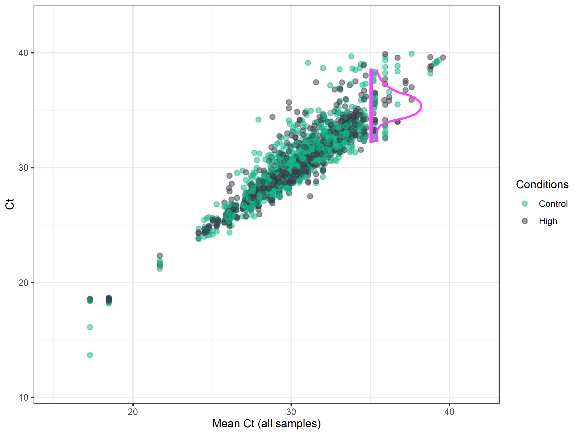
The first step is to decide the Ct cut-off for reliable measurements, as accuracy tends to decrease at high cycle numbers. Then, all missing values and values above the cut-off are replaced by randomly drawn values from a normal distribution that has a mean of the Ct cut-off and a standard deviation of the original data surrounding this cut-off. For example, in the image above, the Ct-cutoff was chosen to remain at the default of 35. Then, values are randomly drawn from the distribution of the data around this point.

Why are some genes removed from the data?

Genes are removed either because the well filter, or if there were too few values for differential expression analysis. The filter is determined by the "Filter wells" drop-down menu on the normalization page. It is for removing QC wells and for automatically detecting likely outlier measurements.

ANOVA and Kruskal Wallis do not work with less than three replicates per condition, and so genes with two or fewer replicates for any experimental condition are removed. This issue is not encountered if missing values are imputed. You can see which genes are removed using the processing summary table.

Which statistical method to use for differential analysis?

Limma is a popular method for differential analysis that was first developed for microarray differential analysis. It addresses the problem of low sample sizes typical to whole-transcriptome studies by using the whole expression profile to make more stable estimates of gene expression variance. EdgeR and DESeq2 were both developed to analyze RNAseq data. All three methods are well-established and should give similar results. Please note:

• EdgeR and DESeq2 are only designed for RNAseq data and will be disabled for microarray data.
• Due to high computational resources required, DESeq2 will be disabled when your dataset contain over 50 samples.

My data contains multiple metadata, how should I choose a proper method for differential analysis?

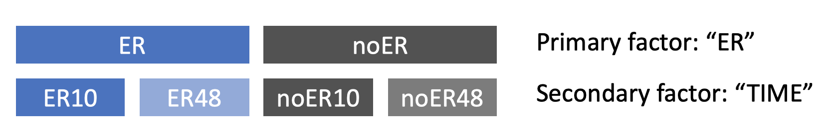
In differential expression analysis, you should first determine whether any of the metadata encode blocking factors, then decide on how to classify individual samples into groups, and finally decide which groups of samples should be compared to each other using statistical tests. Let's assume that none of your metadata are blocking factors (more on that later) and try to understand how selecting primary and secondary factors creates different groups of samples. Consider the "Estrogen" example data, generated in a study that measured gene expression at multiple time points in breast cancer cells in which the estrogen receptor (ER) was either present or absent. Here, the metadata are "ER" and "TIME". As the figure below shows, selecting "ER" as the primary factor divides the data into two groups because "ER" has two different levels ('present' and 'absent'). Selecting "TIME" as the secondary factor results in four groups because the two primary groups are split based on the two time points. If there were three time points, each primary group would be split into three groups, resulting in six groups overall.

The defined groups can now be compared to find genes that are differentially expressed between them (more details on this in later sections). In some experimental designs, we aren't interested in finding the genes that are differentially expressed between the groups defined by the secondary factor because it is a blocking factor. Examples of blocking factors are subject IDs when multiple samples were taken from the same subject (e.g. paired samples, multiple tissue types), or batches of samples that were measured at different times or in different locations. If you indicate that your secondary factor is a blocking factor, EcoToxXplorer will conduct comparisons within the groups that it defines, which typically improves the accuracy of the overall result.

I received the error message "no residual degrees of freedom", what should I do?

This means you do not have enough samples to perform the analysis you specified, usually when combining two metadata in an independent two-factor analysis (no blocking factors). In this case, the total number of groups will be the product of the number of levels in each metadata factor (i.e. if the primary metadata contains 3 levels, and the secondary metadata contains 4, the total number of groups will be 3 * 4 = 12). We recommend a minimum of 3 samples per group, therefore at least 36 samples are required in order to perform a 3 x 4 two-factor analysis.

In this case, you should focus on a single primary metadata and leave the seconday metadata as "Not available", and perform differential analysis with regard to individual metadata. You can then choose the other metadata as the primary metadata and perform the analysis again. If there are no or very few significant genes identified, it is most likely that incorporating the secondary metadata into the analysis will not affect the result.

What are the differences between pair-wise comparisons and time-series comparisons?

A pair-wise comparison tests for genes that are differentially expressed between any pair of groups. For example, take three groups A, B, and C. The "all pairwise" comparison will contrast A-B, A-C, and B-C. A time-series comparison will only contrast consecutive pairs of groups, so in our example only A-B and B-C. Time-series are commonly used when gene expression was measured at multiple time points, or after treatments with varying concentrations/durations.

What is a nested comparison?

A nested comparison allows you to determine which genes respond differently to a treatment condition, respective to some other metadata. For example, consider the experimental design described in the section on multiple metadata where cells with and without an ER were measured at 10hrs and at 48 hrs. To find the genes that respond differently over time in the ER vs. noER cells, you would perform a nested comparison. First, compare ER10-ER48 to find the genes that are differentially expressed in cells with an ER (ERgenes). Next, compare noER10-noER48 to find the genes differentially expressed in cells with no ER (noERgenes). Finally, to find the genes that respond differently over time in ER vs. noER cells, compare ERgenes-noERgenes.

Selecting "Interaction only" will return significant results from only the ERgenes-noERgenes contrast. Otherwise the full model is returned, which is the combination of significant genes from the ER10-ER48, noER10-noER48, and the ERgenes-noERgenes contrasts.

How are gene-level benchmark doses (BMDs) calculated?

Gene-level BMDs are calculated using six steps.

1. Multiple statistical models are fit to the gene expression values for each gene
2. The model fits are filtered to remove poor fits using the lack-of-fit p-value
3. From the remaining fits, the best-fit model for each gene is selected, thus different genes can have different best-fit models
4. Benchmark responses are computed for each gene based on the expression of the control samples
5. The BMD is calculated as the dose that corresponds to the benchmark response
6. BMDs are filtered to remove those with low confidence

More details are given for each of these steps in the below FAQs.

Where do the statistical models come from and what are their exact equations?

The statistical models are the same models the the US Environmental Protection Agency and the National Toxicology Program have used in their studies on 'omics dose-response analysis. They are the same models available in BMDExpress, and are the ones recommended in the peer-reviewed report that outlines the National Toxicology Program Approach to Genomic Dose-Response Modeling. Exp2 - Exp4 are four different forms of exponential models. Poly2, Poly3, and Poly4 are polynomial models with degree 2, 3, and 4. More details and the full mathematical forms can be found in the NTP report linked above.

Which statistical models should I select?

The NTP recommendations say to use all of the models other than Poly3 and Poly4. While these higher degree polynomials often give good fits, there are concerns that allowing too many changes of direction may over fit the data. However, of the remaining models (Exp2-5, Linear, Polynomial degree 2, Power, and Hill), only Poly 2 allows for non-monotonic behaviour. Thus, if you expect non-monotonic behaviour, you may wish to include higher order polynomials. The NTP report suggests that future implementations of dose-response software should include the ability to constrain Poly3 and Poly4 models to only change direction once. We plan to include this feature in future updates to EcoToxXplorer.

What is a lack-of-fit p-value and which threshold should I choose?

A statistical model has a "lack-of-fit" if it fails to adequately explain the relationship between the x (dose) and y (response) variables. In a lack-of-fit statistical test, the null hypothesis is that the model fits the data. Thus, in these tests a significant p-value indicates that there is evidence that the model does not adequately explain the data, and so here we check that the p-value is greater than the significance threshold . Significance thresholds commonly range from 0.05 to 0.5 depending on the desired stringency. The NTP recommendations give a threshold of 0.10.

How is the best fit model selected for each gene?

After applying the lack-of-fit p-value threshold, there may be several statistical models that fit the data well. From these remaining models, the one with the lowest AIC (Akaike information criterion) is selected as the best fit. The AIC is a measure of prediction error that penalizes models with more parameters. This means that if there are two models that do an equally good job of explaining the data, the model with fewer parameters will be selected.

The AIC is not displayed in the results table on the curve fitting page, but it is included in the bmd.csv file that can be downloaded from the Analysis Pipeline side panel.

What is the BMR factor?

BMR means "benchmark response", which is the pre-determined response level that is considered "adverse" or "significant". The dose that corresponds to the BMR is defined as the benchmark dose (BMD). In an ideal case, we would know which change in response variable is physiologically significant and potentially toxic, however this is rarely known for individual genes. For 'omics dose-response analysis, the NTP recommended approach defines the BMR for a gene as the mean of the control gene expression values, plus or minus a certain number of standard deviations of the control values. The number of standard deviations is the BMR factor, and increasing this parameter increases the absolute value of the BMR for each gene.

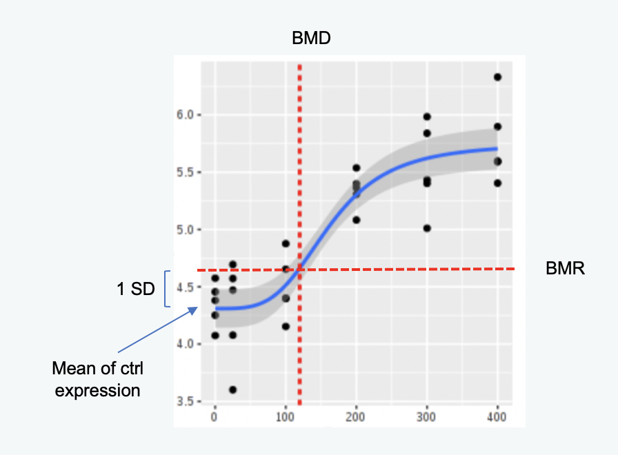
In the figure above, the BMR factor is one since this is the number of standard deviations that was used to calculate the BMR.

How are the BMD_l and BMD_u calculated for each gene?

The BMD_l and BMD_u are the lower and upper limits of the 95% Wald confidence interval of the BMD, extracted from the model-fit object. The BMD_l is sometimes used instead of the BMD since it is a more conservative estimate that depends on the uncertainty of the model fit to the data.

Why are there some genes with model fits but no BMDs?

There are several quality criteria applied to the BMDs to filter out low-confidence or otherwise undesirable BMD estimates:

• Confidence interval width: a wide confidence interval indicates a low-confidence estimate of the BMD. BMDs are eliminated if the BMD_u/BMD_l is greater than 40.
• High dose extrapolation: BMDs that are higher than the highest dose are sometimes due to unpredictable model behaviour beyond the measured data (especially with higher order polynomials). BMDs are eliminated if they are greater than the highest dose.

Additionally, for some genes, the expression values never exceed the BMR and thus EcoToxXplorer cannot compute a BMD.

What is a transcriptomic POD and how is it calculated?

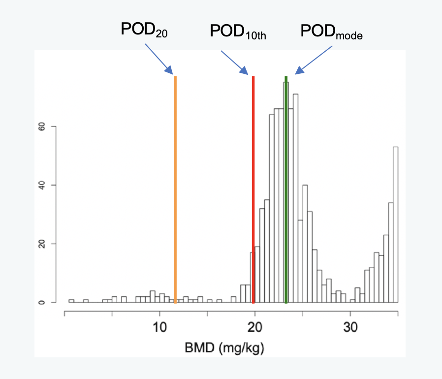
The intial curve fitting and BMD calculation are done at the gene level (geneBMD). However, the main statistic of interest is usually the dose at which the whole-transcriptome is responding to chemical exposure, or the tPOD. The NTP report defines the tPOD based on pathway enrichment analysis of the geneBMDs. However, with many ecological species these pathway-based tPODs are unstable due to the low number of annotated gene sets compared to popular mammalian model organisms, and thus it has been proposed to estimate a statistical tPOD based on the distribution of geneBMDs. There are two different methods for estimating statistical tPODs in EcoToxXplorer:

• tPOD_10th: the tPOD is equal to the 10th percentile of the geneBMD values
• tPOD_mode: the tPOD is equal to the mode of the first peak in the distribution of geneBMD values

How are pathway BMDs (pathBMDs) calculated?

Gene set analysis is used to identify significantly overrepresented pathways in the list of geneBMDs. Pathway-level BMDs (pathBMDs) are calculated as the bootstrapped median of the geneBMDs in that pathway. The National Toxicology Program Approach to Genomic Dose-Response Modeling defines the omicBMD as the lowest pathBMD.

What do the colours on the pathway heatmaps represent?

The pathway heatmap values are calculated through a series of steps:

1. The fitted model for each gene is evaluated across the range of doses in the uploaded data.
2. The resulting modeled expression values are normalized by subtracting the minimum and then dividing by the maximum, producing a set of numbers between zero and one.
3. Genes with a BMD that is down-regulated compared to the control are identified. Their values are inverted by subtracting 1 and then multiplying by -1, which creates a consistent colour gradient from blue on the left to red on the right. The direction of regulation is noted by the coloured boxes on the left side with red for up-regulated and green for down-regulated.
4. Genes are ordered by their BMD.
5. The heatmap cells where geneBMDs fall are coloured black.

The purpose of these steps are to produce a visually appealing heatmap that clearly shows how the expression of each pathway gene compares to the others.

What fold-change values are displayed in the visualizations?

By default, fold-change values are from the comparison selected on the "Feature Selection" page. To use the interactive visual analytics tools to view other results, navigate back to this page and update the drop-down menu.

What algorithm is used for gene set enrichment analysis?

All gene set analysis in EcoToxXplorer is over-representation analysis, computed using hypergeometric tests. This test computes the probability that the list of differentially expressed genes contains more results from a particular gene set than would be expected if the list of DEGs were drawn randomly. EcoToxXplorer supports gene set analysis of EcoToxModules and EcoToxProcesses. Other gene set libraries such as Gene Ontology do not contain enough representation from each pathway since the EcoToxChips have only 384 wells. Since the EcoToxModules and Processes are much larger, this is less of an issue.

How do I change the genes in the heatmap focus view?

You can drag your mouse over a section of the smaller overview on the left side of the heatmap page. The section that you highlight will appear in the focus view. Since gene set analysis is generally performed on the focus view, this allows you to visually identify clusters of genes with distinct expression patterns, view them in more detail in the focus view, and try to understand which biological processes they represent using enrichment analysis.

How were the EcoToxModules defined?

The following steps were taken to define the EcoToxModule gene sets:

1. Choosing biological processes that are relevant to ecotoxicology (the EcoToxModules) that fall into five larger categories (the EcoToxProcesses)
2. Sorting individual KEGG pathways into appropriate EcoToxModules
3. Annotating transcripts from the six EcoToxChip species with KEGG IDs using the KofamScan software
4. Assigning EcoToxChip genes to EcoToxModules if their transcripts were annotated with KEGG IDs that belong to the selected pathways
5. Manually considering the EcoToxChip genes to add any obvious module assignments that were missing. For example, KEGG pathways for vertebrates were based off mammalian species, and so do not contain vitellogenin. We manually assigned this important toxicology biomarker to "Endocrine - Reproduction".

See more details here ...

How is the color of the EcoToxChip rectangle on the Sankey plot determined?

Either the mean or median of the abs(log2FC) for every gene on the EcoToxChip is computed to get a summary score for the whole chip. The colour is then determined by comparing it to the thresholds. This is the same method that is used to determine the colour for each process and module.